Explore penguins

Roland Krasser

2024-12-06

How to explore the penguins dataset using the explore package.

The explore package simplifies Exploratory Data Analysis (EDA). Get faster insights with less code! We will use < 10 lines of code and just 6 function names to explore penguins:

function	package	description
library()	{base}	load a package
filter()	{dplyr}	subset rows using column values
describe()	{explore}	describe variables of the table
explore()	{explore}	explore graphically a variable
explore_all()	{explore}	explore all variables of the table
explain_tree()	{explore}	explain a target using a decision tree

The penguins dataset comes with the palmerpenguins package. It has 344 observations and 8 variables. (https://github.com/allisonhorst/palmerpenguins)

Furthermore, we use the packages {dplyr} for filter() and %>% and {explore} for data exploration.

library(dplyr)
library(explore)
penguins <- use_data_penguins()
# equivalent to 
# penguins <- palmerpenguins::penguins

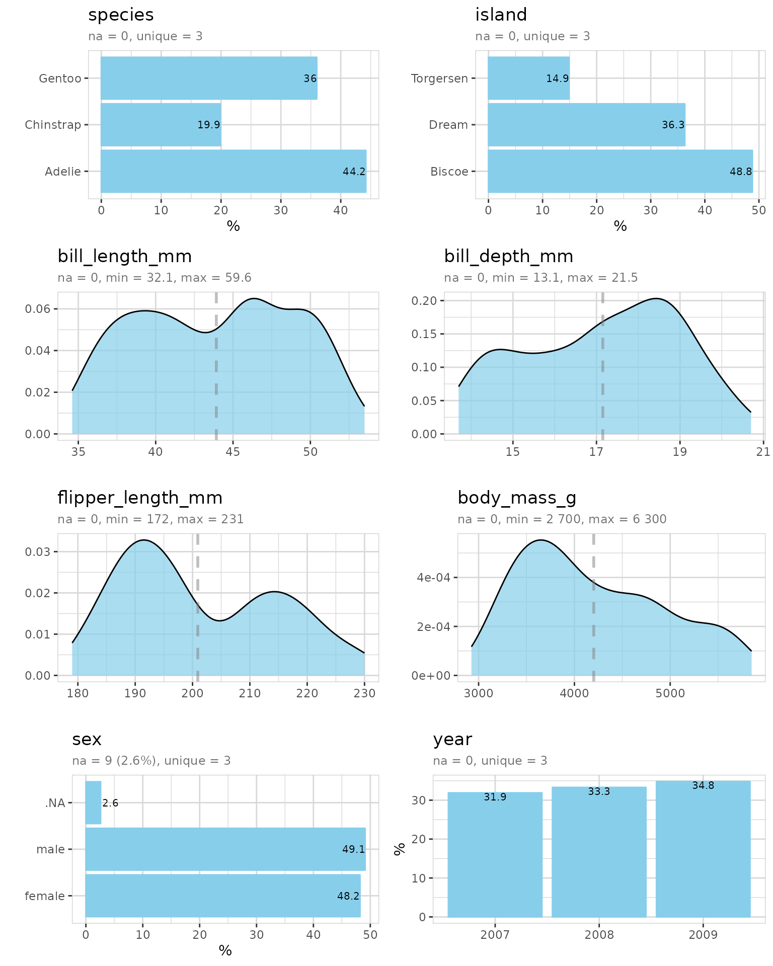
Describe variables

penguins %>% describe()
#> # A tibble: 8 × 8
#>   variable          type     na na_pct unique    min   mean    max
#>   <chr>             <chr> <int>  <dbl>  <int>  <dbl>  <dbl>  <dbl>
#> 1 species           fct       0    0        3   NA     NA     NA  
#> 2 island            fct       0    0        3   NA     NA     NA  
#> 3 bill_length_mm    dbl       2    0.6    165   32.1   43.9   59.6
#> 4 bill_depth_mm     dbl       2    0.6     81   13.1   17.2   21.5
#> 5 flipper_length_mm int       2    0.6     56  172    201.   231  
#> 6 body_mass_g       int       2    0.6     95 2700   4202.  6300  
#> 7 sex               fct      11    3.2      3   NA     NA     NA  
#> 8 year              int       0    0        3 2007   2008.  2009

There are some NA-values (unknown values) in the data. The variable containing the most NAs is sex. flipper_length_mm and others contain only 2 observations with NAs.

Data cleaning

We use only penguins with known flipper length for the data exploration!

data <- penguins %>% 
  filter(flipper_length_mm > 0)

We reduced the penguins from 344 to 342.

Explore variables

data %>% 
  explore_all(color = "skyblue")

Which species?

What is the relationship between all the variables and species?

data %>% 
  explore_all(
    target = species,
    color = c("darkorange", "purple", "lightseagreen"))

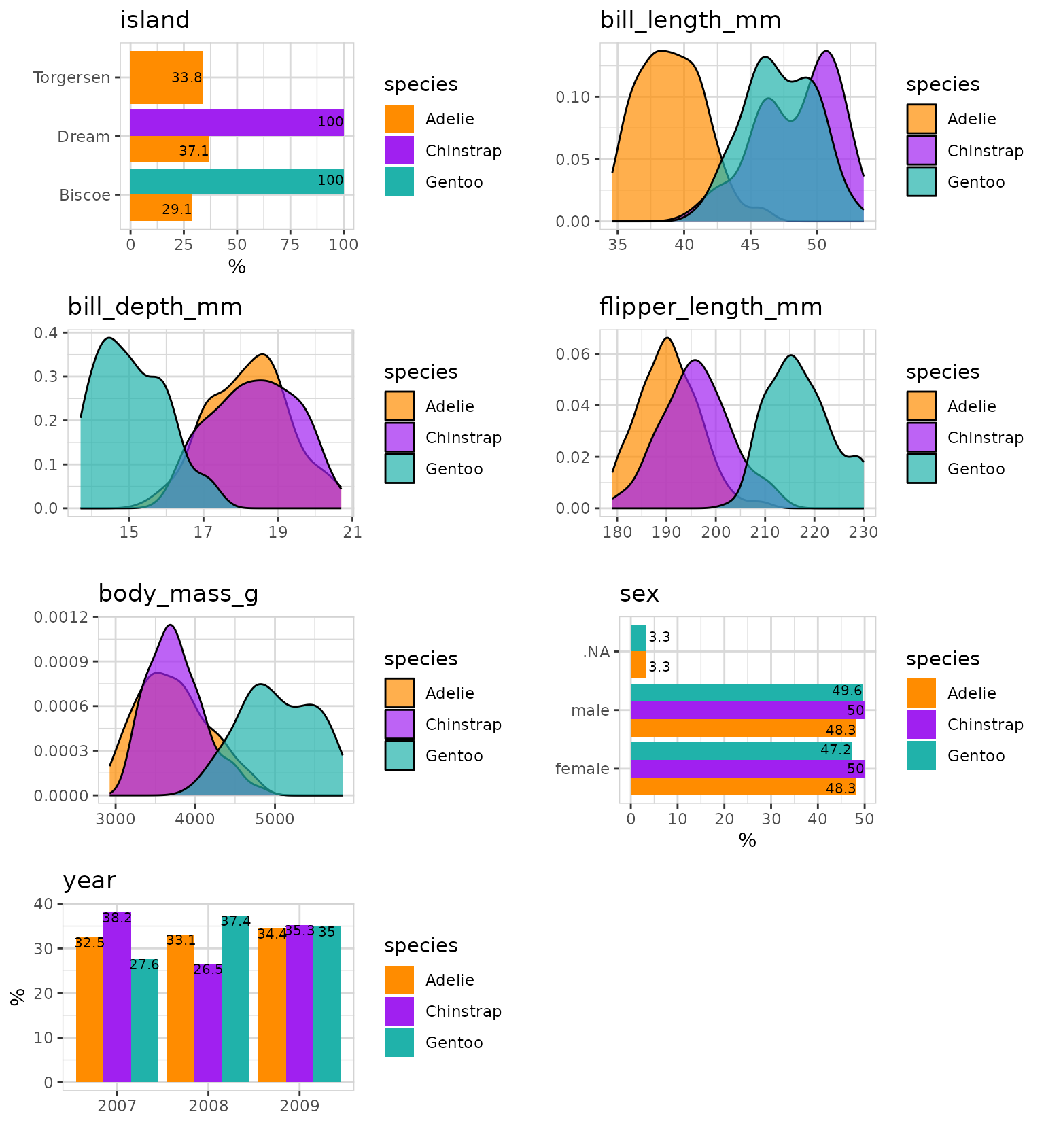
We already see some strong patterns in the data. flipper_length_mm separates species Gentoo, bill_length_mm separates species Adelie from Chinstrap. And we see that Chinstrap and Gentoo are located on separate islands.

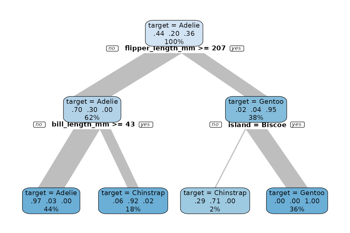
Now we explain species using a decision tree:

data %>% explain_tree(target = species)

We found an easy explanation how to find out the species by just using flipper_length_mm and bill_length_mm.

• If flipper_legnth_mm >= 207, it is a Gentoo penguin (95% right)
• If flipper_length_mm < 207 and bill_length_mm < 43, it is a Adelie penguin (97% right)
• If flipper_length_mm < 207 and bill_length_mm >= 43, it is a Chinstrap penguin (92% right)

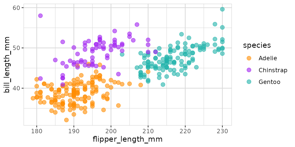
Now let’s take a closer look to these variables:

data %>% 
  explore(
    flipper_length_mm, bill_length_mm, 
    target = species,
    color = c("darkorange", "purple", "lightseagreen")
    )

The plot shows a not perfect but good separation between the 3 species!