
Let's {explore} count-data!
{explore} simplifies Exploratory Data Analysis (EDA) … now you can use {explore} with count-data too! Let’s take a look at the Titanic dataset!
What are count-data?
Data are stored in tables most of the time. This data is called tidy if:
- Each row is an observation
- Each column is a variable
- Each cell is a value
So in a tidy Titanic-dataset each row is representing a person on the ship. Each column is representing a variable (like age or gender). And each cell is representing a value (like the gender of a specific person is “Male”)
titanic_tidy
# A tibble: 2,201 x 5
      id Class Sex   Age   Survived
   <int> <fct> <fct> <fct> <fct>
 1     1 3rd   Male  Child No
 2     2 3rd   Male  Child No
 3     3 3rd   Male  Child No
 4     4 3rd   Male  Child No
 5     5 3rd   Male  Child No
 6     6 3rd   Male  Child No
 7     7 3rd   Male  Child No
 8     8 3rd   Male  Child No
 9     9 3rd   Male  Child No
10    10 3rd   Male  Child No
# ... with 2,191 more rows
We see that the first 10 observations are similar except the id. So the basic idea of having count-data is, to group all similar observations and add a count variable. Let’s use the Titanic dataset that comes with Base R:
library(tidyverse)
titanic <- as_tibble(Titanic)
# A tibble: 32 x 5
   Class Sex    Age   Survived     n
   <chr> <chr>  <chr> <chr>    <dbl>
 1 1st   Male   Child No           0
 2 2nd   Male   Child No           0
 3 3rd   Male   Child No          35
 4 Crew  Male   Child No           0
 5 1st   Female Child No           0
 6 2nd   Female Child No           0
 7 3rd   Female Child No          17
 8 Crew  Female Child No           0
 9 1st   Male   Adult No         118
10 2nd   Male   Adult No         154
# ... with 22 more rows
Now we have a table with just 32 rows instead of 2201 without any lost of information!
Count-data:
- Each row is a group of observations with similar attributes
- One column is a numeric variable representing the number of observations
- The rest of the columns are categorical variables
- Each cell is a value
So, what is the benefit of using count-data instead of tidy-data? Using count data will save a lot of memory and disk space and you will explore the data much faster!
| Titanic dataset | rows | file size csv |
|---|---|---|
| tidy-data | 2201 | 85 KB |
| count-data | 32 | 2 KB |
| 1.5% | 2.4% |
For the Titanic-data it may not make much a difference, as the data is small anyway. But if you think of a dataset with millions of observations but low number of variables or low variation in the data, using count data will save a lot of memory and disk space and you will explore the data much faster! Generating count-data from tidy data is something that a classic datawarehouse or any relational database can do very fast and efficient.
Describe count-data
We can use {explore} to take a closer look to the data:
library(tidyverse)
library(explore)
titanic <- as_tibble(Titanic)
titanic %>% describe()
# A tibble: 5 x 8
  variable type     na na_pct unique   min  mean   max
  <chr>    <chr> <int>  <dbl>  <int> <dbl> <dbl> <dbl>
1 Class    chr       0      0      4    NA  NA      NA
2 Sex      chr       0      0      2    NA  NA      NA
3 Age      chr       0      0      2    NA  NA      NA
4 Survived chr       0      0      2    NA  NA      NA
5 n        dbl       0      0     22     0  68.8   670
Thera are 5 variables in the data, the variable n is representing the number of the observations. To take a look at the size of the “uncounted” data, we can simply:
titanic %>% describe_tbl(n = n)
2 201 (2.2k) observations with 5 variables
0 observations containing missings (NA)
0 variables containing missings (NA)
0 variables with no variance
We see that the 32 rows of the data contains 2201 observations and 5 variables (one is containing the number of observations)
Explore count-data
We can visually explore a variable of the count-data simply using the explore function:
titanic %>%
  explore(Class, n = n)
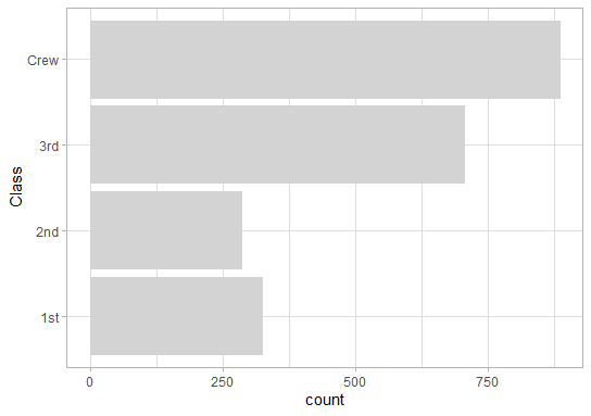
So about 40% of all people on the Titanic were Crew-Members!
We can visually explore the relationship between a variable and a target:
titanic %>%
  explore(Class, target = Survived, n = n)
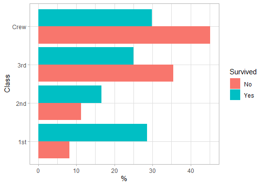
Bars of the same color sum up to 100%. If there is a large difference in bar-length between colors, there is an interesting pattern. So Crew Members had a much lower chance to survive than Passengers in 1st class.
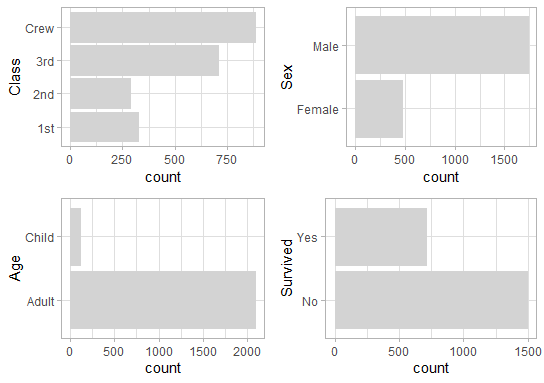
We can even explore all variables in one line of code:
titanic %>%
  explore_all(n = n)
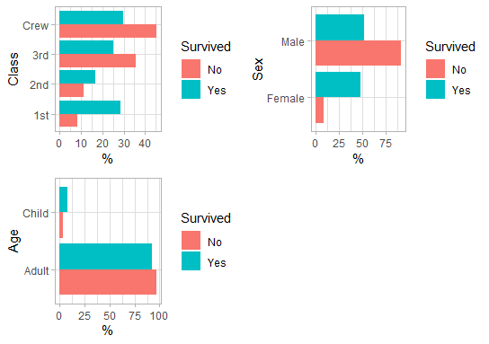
And the relationship of all variables with a target:
titanic %>%
  explore_all(target = Survived, n = n)
Report count-data
We can generate a rich HTML-report with just one line of code:
titanic %>%
  report(n = n, output_dir = tempdir())
To get a reoprt of the relationship between all variables and the target:
titanic %>%
  report(target = Survived, n = n, output_dir = tempdir())
Explain a target
We can create a simple decision tree to explain a target (in our case Survived)
titanic %>%
  explain_tree(target = Survived, n = n)
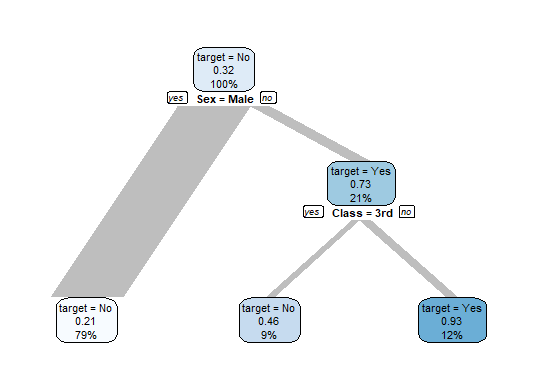
So, overall 32% of the people survived. This is shown in the top-node. “target = No” means that the majority (50% or more) of passengers did not survive. 0.32 is the proportion of passengers that survived (32%) and 100% is the percentage of all passengers that are in this node.
Splitting by Gender already shows a strong pattern: only 21% of all male survived, but 73% of all female. Taking a closer look to females, we see that better classes had better chances to survive (46% of 3rd class survived, but 93% of better classes)
Links
{explore} is on CRAN
There you find some more examples how to use it: